In the realm of medicine, before we understood germs it was only natural to assume illness was caused by the wrath of the “gods”, “curses” or “ghosts in your blood” and bloodletting seemed like a natural solution. Enter modern medicine with its framework for understanding disease through germ theory. We no longer relied on stories of disease being caused by omnipotent beings or vengeful fairies but had a clear mechanism that could be tested.

The same applies in economic and finance. Without a solid framework for thinking about what causes a given phenomenon (inflation, interest rates, recessions, etc), it’s only natural that people will resort to their own ad hoc explanations for what “causes” these phenomena. That’s where you get errors: confusing correlation for causation, mistaking an accounting identity for an economic mechanism, or treating a compelling story as if it were evidence. The field of finance and economics should be able to provide people with simple (but not simplistic) frameworks for how to think about things like interest rates, prices, inflation, so that we can think, talk and discuss issues related to them in a common language.

Questions like, why do house prices vary over time or across cities? Why do prices of goods and services vary over time? Why do stock prices go up and down? Why are interest rates high in one country and low in another? All need a framework from which to properly understand them. So much debate in the media sees to stem from a lack of common framework.

Take stock prices. If you asked the average person on the street, they would give you all sorts of strange ad-hoc explanations for what moves stock prices. Finance gives you a compact, surprisingly useful starting point: a stock price is the market’s best guess of future cashflows, discounted for time and risk (a topic for a future post). That single sentence immediately disciplines the conversation. If stocks fall, you are basically saying at least one of three things changed: expected cashflows, the risk-free rate, or the compensation investors demand for bearing risk. You can still disagree—strongly—about which of those moved, but you’re no longer explaining prices with “ghosts in the blood” type thinking.

Having a framework does not mean that we can predict the future or that frameworks never change. Frameworks adapt and evolve over time as does our understanding. Physics has its own framework for thinking about how atoms and the fundamental forces in the universe work (it’s called the Lambda-CDM model). It’s the result of the cumulative work of centuries of scientists studying the universe and trying to develop a framework that explains the behaviour of everything we see from electromagnetism to the structure of galaxies. However, this framework is almost certainly incomplete (the current framework cannot reconcile gravity with quantum mechanics).

Frameworks give us a conceptual structure to organise our thinking, understand the world and frame certain questions to improve the framework. They do not give us a crystal ball to predict the future.

This series is my attempt to articulate those frameworks. It’s not that this knowledge is new. Economics and finance, as professions, have accumulated a set of useful frameworks over decades. But we often do a poor job of communicating them. We forget that people who are not immersed in thinking about these topics every day, can look at economics and finance from the outside, and conclude, “these people have no idea what the f$^k they are talking about”. When we don’t have a shared framework, we default to intuitive stories. Sometimes they’re right; often they’re not. My premise is that it’s a communication issue, not a content issue.

In this series I’m going to lay out a small set of “workhorse” frameworks for thinking about concepts like prices, inflation, interest rates, and other ideas in economics and finance. The goal is to build a common language that helps you spot bullshit faster, argue more rigorously, and think more clearly.

In this post I will explain how to calculate the Distance to Default (DtD) using the Merton model in R. The DD measures how many standard deviations the firm’s asset value is away from the default point, providing a summary of the firm’s credit risk.

To implement the Merton DtD model in R, I have drawn inspiration from the SAS code provided by Bharath and Shumway (2008) and the methodologies discussed by Mingze Gao. The process involves estimating the firm’s asset value and its volatility iteratively, then calculating the DtD based on these estimates.

Step 1: Setting Up the Environment

The script starts by clearing the environment and setting options for numerical precision:

rm(list=ls())  # Clear all user-defined objects
options(digits=4, stringsAsFactors = FALSE, scipen=999)  # Set numerical precision

Then, it loads necessary libraries:

library(tidyverse)
library(dplyr)
library(tidyr)
library(roll)

These packages are essential for data manipulation, time series calculations, and rolling-window statistics.

Step 2: Loading and Preparing Data

2.1 Load CRSP/COMPUSTAT Daily Data

The script loads daily stock market data from CRSP/COMPUSTAT and calculates market equity (E) and rolling volatility:

ccm_data <- read.csv("crsp_compustat_daily_sascha.csv") %>%
  mutate(datadate = as.Date(datadate, format = "%d/%m/%Y")) %>%
  mutate(E = cshoc * prccd) %>%  # Market value of equity
  group_by(GVKEY) %>%
  mutate(returns = (prccd - lag(prccd, 1)) / lag(prccd, 1)) %>%
  mutate(sigma_E = roll::roll_sd(returns, width = 252, min_obs = 30))

The sigma_E variable represents the rolling standard deviation of stock returns, which approximates equity volatility.

2.2 Load Quarterly COMPUSTAT Data

Quarterly firm liabilities (debt) are imported and interpolated:

cmp_data <- read.csv("compustat_qtrl_sascha.csv") %>%
  mutate(date = as.Date(datadate, format = "%d/%m/%Y")) %>%
  mutate(F = (dlcq + dlttq) * 1000000) %>%  # Total firm debt
  fill(F, .direction = "down") %>%  # Forward-fill missing values
  replace_na(list(F = 0))  # Set missing values to zero

The debt values are joined with the daily dataset and forward-filled between quarters.

2.3 Load Risk-Free Rate Data

The script loads and processes 3-month Treasury bill rates:

frb_rates_monthly <- read.csv("frb_rates_monthly.csv") %>%
  mutate(date = as.Date(date, format = "%d/%m/%Y"), r = as.numeric(RIFLGFCM03_N.B) / 100) %>%
  fill(r, .direction = "down") %>%
  mutate(r = ifelse(r == 0, 0.01, r))  # Set zero rates to 0.1%

This provides the risk-free interest rate (r), a key input for the Merton model.

2.4 Data Cleaning and Finalization

The dataset is cleaned and filtered:

panel_data <- ccm_data %>%
  filter(!is.na(sigma_E) & !is.na(E) & !is.na(F) & F > 0) %>%
  mutate(E = E/1000000, F = F/1000000)  # Convert values to millions

Step 3: Implementing the Iterative KMV-Merton Model

The Merton model treats equity as a call option on the firm’s assets. The script estimates asset value (V) and volatility (sigma_V) iteratively:

3.1 Defining the Iteration Function

The function compute_group estimates asset values and default probabilities:

compute_group <- function(hist_data) {
  end_obs <- hist_data %>% filter(date == max(date)) %>% slice(1)
  E_end <- end_obs$E; F_val <- end_obs$F; r_val <- end_obs$r; sigma_E_val <- end_obs$sigma_E
  sigma_V <- sigma_E_val * E_end / (E_end + F_val)  # Initial guess

  iter <- 0; tol <- 1e-3; max_iter <- 100
  repeat {
    iter <- iter + 1
    solve_V <- function(E_daily) {
      f_equity <- function(V) {
        d1 <- (log(V/F_val) + (r_val + 0.5*sigma_V^2)) / (sigma_V)
        d2 <- d1 - sigma_V
        V * pnorm(d1) - exp(-r_val) * F_val * pnorm(d2) - E_daily
      }
      uniroot(f_equity, lower=F_val, upper=10*E_daily)$root
    }
    V_series <- map_dbl(hist_data$E, solve_V)
    sigma_V_new <- sqrt(252) * sd(diff(log(V_series)), na.rm=TRUE)
    if (abs(sigma_V_new - sigma_V) < tol || iter >= max_iter) break
    sigma_V <- sigma_V_new
  }

  V_end <- tail(V_series, 1)
  DD_val <- (log(V_end/F_val) + (r_val - 0.5 * sigma_V^2)) / sigma_V
  EDF_val <- 100 * pnorm(-DD_val)
  tibble(V=V_end, sigma_V=sigma_V, DD=DD_val, EDF=EDF_val, iterations=iter)
}

This function estimates:

• V: Firm’s asset value
• sigma_V: Asset volatility
• DD: Distance to Default (DtD)
• EDF: Expected Default Frequency

A safe wrapper ensures errors return NA values.

3.2 Applying the Model Firm-by-Firm

The iterative procedure is applied to all firms:

results <- panel_data %>%
  group_by(gvkey) %>%
  arrange(date) %>%
  group_modify(~ {
    tibble(date = unique(.x$date)) %>%
      mutate(calc = map(date, ~ safe_compute_group(filter(.x, date <= . & date >= . - 365)))) %>%
      unnest(calc)
  }) %>%
  ungroup()

The function calculates DtD for each firm, using a 365-day rolling window.

Step 4: Exporting the Results

Finally, the computed results are saved:

write.csv(final_results, "updated_dtd.csv")

This file contains firm-level DtD values over time

Lets look at two examples. Example 1, a game of Russian Roulette. Imagine a game where one bullet is loaded into a six-chamber gun. If you play, and the barrel lands on an empty chamber, you win $1million. If the barrel lands on the chamber with a bullet, you die. Now let’s say you have 6 people, who each play the game once. 5 people, or 83% of players turn out to be millionaires, and one unlucky person dies. Would you take that bet? Now imagine a slightly different game. Instead, just one person plays, but the same person plays 6 rounds. Still seem like an enticing game?

Let’s look at another example. Imagine a game where you roll a die and win or lose money based on the outcome. The rules are: Rolling a 1, 2, or 3: Lose $10. Rolling a 4, 5, or 6: Win $10. What is the time average (i.e. the average of a single player over time)? Say you play the game 100 times and record your winnings. Your time average is the average outcome of your rolls over these 100 games. For example, if the first five roll outcomes are (1,6,3,4,2), your winnings after five rounds would be −$10 + $10 − $10 + $10 − $10 = -$10. After one hundred rounds, your average winnings may differ significantly depending on the sequence of rolls.

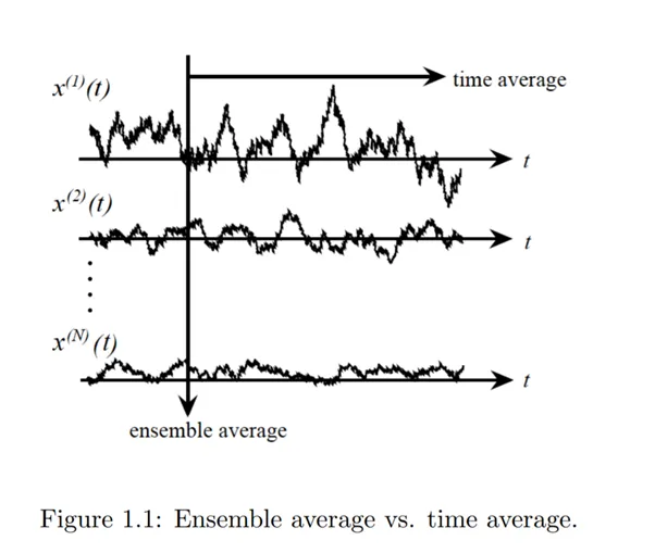
What is the ensemble average (i.e. the average over many players at once)? Now imagine 1,000 players each rolling the die once. The ensemble average is the average outcome across all players. If it is a fair die, half the players roll 1, 2, or 3 and lose $10, while the other half roll 4, 5, or 6 and win $10. The ensemble average is (−$10 x 500 + $10 x 500 ) / 1000 = $0.

The key difference being that the ensemble average gives a neutral expectation ($0 in this case), assuming all outcomes occur equally across players. Whereas the time average depends on the specific sequence of rolls for an individual player and may differ from the ensemble average.

Stock returns also exhibit such non-ergodic behaviour. We can see the impact this has on a portfolio using a simulation in R. The simulation below creates two portfolios and tracks their value over time from time period 0 to time period 100. The initial investment is $100. I generated as list of 100 random returns (from -20% to +20). Both portfolios use the same 100 random returns, but in different orders. The figure below plots one iteration of the value of the portfolios over time:

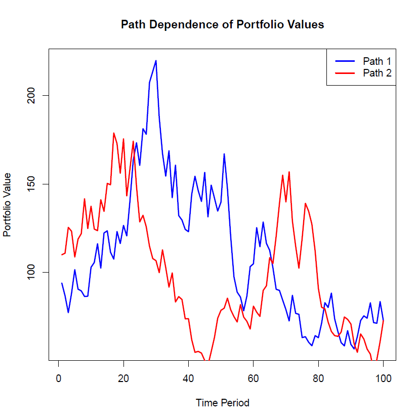
We see the paths of the two portfolios can diverge significantly over time due to differences in the sequence of returns, even when the same set of returns is applied in a different order. If you happen to be retiring in year 50, the performance of your portfolios could vary greatly, leading to vastly different outcomes. This underscores the critical importance of considering sequence-of-returns risk when constructing investment portfolios. Since non-ergodicity penalizes large losses more than it rewards equivalent gains, prioritizing wealth preservation is essential. Safeguarding capital ensures that investors can continue to participate in future growth opportunities.

The code:

# Parameters
n_periods <- 100
initial_investment <- 100

# Simulate two paths of returns
returns_path1 <- runif(n_periods, min = -0.20, max = 0.20) # Random returns between -20% and +20%
returns_path2 <- sample(returns_path1) # Same returns, different order

# Calculate portfolio values over time
portfolio_values_path1 <- cumprod(1 + returns_path1) * initial_investment
portfolio_values_path2 <- cumprod(1 + returns_path2) * initial_investment

# Arithmetic average returns for both paths
arithmetic_avg_path1 <- mean(returns_path1)
arithmetic_avg_path2 <- mean(returns_path2)

# Final portfolio values
final_value_path1 <- tail(portfolio_values_path1, 1)
final_value_path2 <- tail(portfolio_values_path2, 1)

# Output results
cat("Path 1: Final Value =", final_value_path1, "\n")
cat("Path 2: Final Value =", final_value_path2, "\n")
cat("Arithmetic Average Return (Path 1) =", arithmetic_avg_path1, "\n")
cat("Arithmetic Average Return (Path 2) =", arithmetic_avg_path2, "\n")

# Plot the paths
plot(1:n_periods, portfolio_values_path1, type = "l", col = "blue", lwd = 2, 
     xlab = "Time Period", 
     ylab = "Portfolio Value", 
     main = "Path Dependence of Portfolio Values")
lines(1:n_periods, portfolio_values_path2, col = "red", lwd = 2)
legend("topright", legend = c("Path 1", "Path 2"), col = c("blue", "red"), lwd = 2)

#Descriptive
summary(portfolio_values_path1)
summary(portfolio_values_path2)

To really understand this issue there are a couple principles which need to be understood. First, what is the difference between inflation and the price level? Second, what is the difference between relative prices and the price level. Much confusion about inflation can be explained by confusion about the definition of these, as pointed out by John Cochrane.

The first question is what is inflation? This might seem obvious, but inflation is the growth rate of general prices within an economy. This is different from the price level. The price level refers to the overall average level of prices at a given time, while inflation measures the rate of change in the level over time. The average level of prices in the economy is typically measured by a government agency, who go out and survey the price of 1000’s of goods and services around the country. In Australia, that job is performed by the Australian Bureau of Statistics (ABS) which measures prices at a monthly level (although every quarter they do a more detailed survey). The ABS then create a price index which tracks the average price of goods/services over time. This is a measure of the price level. The rate of change in the price level (typically measured as the rate of change from 12 months prior) is the inflation rate. When the level of prices is increasing, this is referred to as inflation. If the level of prices is decreasing, this is referred to as deflation. If the rate of inflation is falling, this is referred to as disinflation.

The most widely known measure of inflation is the headline Consumer Price Index (CPI). This includes the rate of change of prices of a representative basket of goods and services (that a consumer would typically purchase). Now all of us spend our money differently, which means that each of us has our own personal inflation rate that we experience. The headline CPI reported by the ABS is the inflation rate on a hypothetical basket of goods/services that is meant to represent the average household (the hypothetical basket does change over time, more details can be found here. There can be different measures of the price level and inflation rate, depending on what prices you decide to include or exclude. For example, the ABS also computes a trimmed mean CPI, or “Core” CPI, which excludes volatile prices like petrol and groceries. The reason being that the prices of these goods are typically driven by global commodity prices, something the central bank cannot control. The trimmed mean CPI gives a “cleaner” measure of the underlying inflation in the economy.

The second key idea is the difference between relative prices and the price level. Relative prices are a measure of the relative prices between two goods, say apples and petrol. Relative price changes occur when one specific good, like petrol, becomes more expensive compared to the price of apples and vice versa. Rising petrol prices alone, are not necessarily a sign of inflation, but indicate a relative price change compared to the price of other goods. Inflation involves a simultaneous rise in the price of all goods and services across the economy, maintaining the same relative price among all goods and services. This leads us to our first takeaway, a price rise in one good or service, is not always a sign of inflation (I’ll explain why below). In true inflation, all goods and services—including petrol and apples—would rise roughly proportionally, preserving their relative price relationships. Inflation is thus a broad monetary phenomenon, not just a summation of individual price increases. Let’s look at the implications of relative price changes. A rise in one sector’s prices (e.g., petrol) will typically lead to a price decrease in other goods. Think about it this way, I have $100 of income to spend between apples and petrol. If the price of petrol goes up this month, I have less money left to buy apples (at least in the short run this is true unless someone gives us more money, i.e. the government through fiscal or monetary policy). Demand and therefore the price of apples will fall. A change in relative prices, all else equal, will keep the overall price level constant, as the price increase of any one good is offset by price falls in the other goods.

This leads to our second takeaway, something that drives a change in relative price, does not cause inflation (on it’s own). For example, the favourite bogeyman of the media is corporate price gouging. If a firm rises the price of a good (beyond some reasonable level relative to costs), this is decried as the root cause of inflation. If only governments could stop firms raising their prices, then inflation could be solved, right? Wrong. It’s the same fallacy as described above. A change in relative prices, means that if the price of one good goes up because a firm is price gouging, leaves consumers with less money to spend on other goods (at least in the short run), keeping the overall price of goods constant. Price gouging can explain changes in relative prices, but it cannot explain inflation across all prices.

So what drives the general price level of all goods and services up simultaneously? In any economic system there must be some force that acts as a reference point or stabilizer for the general price level. In economics there are two such theories which could explain why all prices would move higher, Monetarism and Fiscal Theory of the Price Level. According to Monetarism (of which Milton Friedman was a proponent), the price level is anchored by the supply of money. If the government (through fiscal policy or monetary policy) decides the print a pile of currency and hand it out to people in the form of stimulus checks, consumers will immediately spend that money, bidding up the price of goods and services. This will generate inflation. According to the Fiscal Theory of the price level, government debt’s real value anchors prices. Without a change in the nominal anchor (e.g., more debt or money creation), relative price shifts (e.g., petrol vs. apples) don’t cause overall inflation.

What about supply shocks? Can supply shocks explain inflation? The answer is it depends. For example, if a global pandemic makes it hard to import goods, e.g. Televisions, then the price of these goods will rise. Further compounding this, is lockdowns mean people can’t go out, and instead may buy more televisions instead. But this supply shock is another example of a change in relative prices. If the price of televisions goes up, consumers have less money to spend on other goods, so some other good has to fall in price. So far no inflation. But a supply shock can cause inflation, if monetary and fiscal policy respond to the supply shock. If governments give consumers more money in response to the supply shock, then they will be able to pay the higher price for the televisions without sacrificing spending on other goods. This will lead to inflation. Thats exactly what we saw in 2021 and 2022.

The same logic can be applied to the impact of tariffs on inflation. Will the introduction of tariffs increase the price of some goods (particularly imported goods), yes. That’s a change in relative prices. Unless fiscal or monetary policy provide money, the prices of other goods may fall, leaving overall inflation unchanged.

Market makers, who are typically on the other side of the trade from investors, aim to remain neutral by hedging their exposure to these options. This means that when an investor buys a call option, the market maker sells it to them and might hedge their exposure by purchasing some of the underlying stock to offset potential losses if the stock price rises. Gamma, a measure of the rate of change in an option’s delta (sensitivity to price movement in the stock), becomes crucial here. When there’s a high gamma, it means that the market maker has to continually adjust their hedge—buying more of the stock as it rises or selling as it falls. In a gamma squeeze, large purchases of call options by investors requires market makers to buy up the underlying stock to maintain their delta hedges. This can trigger a feedback loop where rising stock prices force even more stock purchases, leading to dramatic price increases. This “gamma effect” can induce momentum in prices. Academic papers have found strong evidence for this price pressure induced momentum in equities, bonds, commodities, and currencies.

Gamma squeezes typically happen when there’s an unusual spike in call option buying on a specific stock. When gamma squeezes occur, they can lead to exaggerated price movements. This is because market makers, compelled to buy more and more shares as the stock rises, create a self-perpetuating cycle, further fuelling demand for the stock. A recent example is shares in Tesla post-US election, achieving a 30% gain, as noted by the FT

As noted in the article, a wave of call option buying triggering a gamma squeeze is the most likely culprit for this sharp price movement. The notional trading volume in Tesla options has averages $145billion USD a day since the election, peaking at $245billion USD. This is significant, given the entire universe of single-stock options has typical daily volumes of $310billion USD. Other notable examples of previous gamma squeezes include Nvidia and GameStop.

But the implications of option hedging go beyond individual stocks. There is a large market for SP500 index options too. Retail investor purchases of call options could also have contributed to the sharp market rally post-election. This ultimately depends on the position of dealers and their gamma exposure. Beyond gamma, there are other less commonly discussed Greeks, known as “Vanna” and “Charm”. Vanna measures the sensitivity of delta (the option’s price sensitivity to the underlying stock) to changes in implied volatility. It essentially tells us how much delta will change as volatility fluctuates. Vanna measures the sensitivity of delta (the option’s price sensitivity to the underlying stock) to changes in implied volatility. It essentially tells us how much delta will change as volatility fluctuates.

These are particularly relevant given the behaviour of VIX, a measure of implied volatility, around the US election. After the election there was a large drop in the VIX

Depending on the exposure of market makers going into the election, this sharp change in implied volatility, could have also contributed to market makers need to adjust their hedges. If retail investors had purchased large amounts of call options on the SP500, the market makers selling those options would have hedged by selling the underlying futures contract. When implied volatility falls, vanna predicts that the delta of the options will fall, leading the market maker to close out some of their short futures hedges. This buying may further contribute to price pressure in the SP500, above and beyond any “gamma effect”.

A long line of work in the macroeconomic forecasting literature has tested a range of financial variables that have predictive power for economic activity; (See, Friedman1993b, Estrella1991, Gertler2000, Gilchrist2012, Lopez-Salido2017, Mueller2009), but they have typically focused on aggregate data. Saunders et. al 2024 also established that the aggregate loan spread has predictive power for aggregate economic activity above and beyond information contained in bond spreads. But what has been less explored, is if industry-specific loan spreads can predict industry-level economic activity above and beyond information contained in aggregate spreads. I argue the process of aggregating data could obscure useful information for three key reasons.

First, it could be that certain industries are over (or under)-represented in aggregate asset price indexes relative to their true economic contribution. For example, an aggregate loan index (either equal or value-weighted) will place more weight on industries which have more loans outstanding. The figure below plots the sectoral composition of loans and highlights that manufacturing (MAN) and information technology (INFO) have a disproportionate number of loans outstanding relative to other industries. Patterns in MAN and INFO loans spreads will, therefore, have a disproportionate impact on the aggregate loan spread. When compared to the economic contribution of each industry to total gross output (TGO), it is finance (FIN), manufacturing (MAN) and service (SERV) contributing the most to TGO. Therefore, aggregate loan spreads place more weight on industries with more loans outstanding, rather than industries which contribute more to economic activity.

Second, it could be that sectoral shocks are more common than aggregate shocks, and these sectoral shocks would be obscured in aggregate indexes. The figure below highlights recent examples of industry level shocks. The 2001 recession which had its beginnings in the Dot-Com bust, the 2008/9 Global Financial Crisis which had its beginnings in a construction boom, and finally the 2015 Oil-Gas industry collapse following the collapse in the oil price. The blue line indicates the loan spread for the given industry and the black line the aggregate loan spread. This figure reveals that industry specific loan spreads reacted relatively early compared to the loan spreads in other industries around industry-specific shocks. These examples suggests that disaggregated industry level data provided a useful signal about the emerging risks in these particular sectors.

To provide statistics on the incidence of industry-specific shocks, I define a negative shock at the industry level by counting the number of episodes in which the abnormal equity return of an industry is lower than -10%. I define the abnormal return as the industry equity return minus the SP500 return in a given month. The figure below, top panel, highlights there are 52 (industry-month observations) where abnormal equity returns were lower than -10%. Alternatively, I use a 100bps abnormal increase in industry loan spreads as a negative shock. I define the abnormal loan spread as the change in industry loan spread minus the change in aggregate loan spread in a given month. The bottom panel, highlights there are 134 incidences where abnormal industry loan spreads were greater than 100bps. The incidence of negative shocks are more prevalent in certain industries such as ART, AIR, MIN, OIL. Given the frequency of industry-specific shocks, aggregate data may ignore useful signals about emerging risks in the economy.

Third, not all economic shocks are equal. Some shocks affect all industries in the same direction, some affect industries in offsetting directions. For example, the Oil-Gas shock of 2015, was a negative shock for those firms directly linked to the extraction of oil. However, for industries for which energy is a significant input, this same shock was a positive shock. The figure below contrasts the loans spread for the oil and airlines industry. It is apparent the significant drop in oil prices, while negative for one industry, was positive for the other. This example highlights that different types of industry shocks may cancel out in the aggregate.

Given the reasons outlined above, I test whether industry-specific loans spreads contain information that is useful for predicting industry developments, beyond any information contained in the aggregate macroeconomic variables. I adopt the standard forecasting regression framework:

where the dependent variable, \(y\), is either the 1 quarter-ahead growth rate in industry TGO or VA, i.e., the log growth rate in activity from \(t\) to \(t+1\). \(\Delta S_{b,t}\) is the change in industry loan spread from \(t-1\) to \(t\). \(\Delta S_{t}\) is the change in the aggregate loan spread from \(t-1\) to \(t\). All specifications also include one lag of the dependent variable and time or industry fixed effects, depending on the specification.

The table below summarises the baseline result. In column 1 I include only the industry loan spread and find an increase in industry specific loan spreads is associated with a decrease in the growth rate of industry specific output in the next quarter, i.e. a 100bps increase in the industry loan spread is associated with a 8 bps decrease in TGO next quarter. This is statistically and economically significant compared to the unconditional average of 47 bps in TGO growth over the next quarter. To test whether there is additional information in the industry level loan spreads, column 2 includes the aggregate loan spread. The coefficient on the industry spread remains negative and significant. Finally, column 3 includes industry and time fixed effects to absorb any common time trends. Column 4-6 repeat the same set of regressions but use industry VA as the dependent variable. Together, the table suggests industry specific loan spreads contain useful information for predicting industry level economic activity. The results are agnostic as to which component of credit spreads is reacting early. Credit spreads could change because investors are forecasting a deterioration in borrower health, or it might be that risk premia increase. However, given that not all industry spreads are changing simultaneously, this is more consistent with changes in borrower health, than changes in broad investor risk aversion.

One may argue that equity markets, being larger and more liquid, should also contain useful information about predicting industry economic activity. Therefore in the table below, I test the ability of industry equity returns to predict industry economic activity. I repeat the specification used in the previous table, except replacing loan spreads with equity returns. Column 1/2 (4/5) suggest that an increase in equity returns predicts an increase in TGO (VA) in the next quarter. However, note that in column 2 and 5, once controlling for aggregate equity returns (i.e. returns on the SP500), the power of industry equity returns is substantially reduced. Furthermore, with the addition of fixed effects in column 3 and 6, the statistical significance disappears. This suggests that industry specific equity returns do not contain much additional information for forecasting industry level activity beyond the market return.

What is the benefit of using industry level loan spreads and who would find these results useful? First, policy makers would benefit from tracking industry level spreads to obtain a better understanding of the state of the economy. Furthermore, industry spreads may provide insights into the transmission mechanisms of monetary policy by tracking conditions in interest rate sensitive sectors. Second, bank loan officers would be a user of industry information given their role in allocating credit. For example, Blickle et. al (2023) show that loan portfolios of banks do show a tendency to specialise in certain industries. Industry credit spreads would provide loan officers with an additional barometer of conditions in each industry.

The central bank is responsible for setting monetary policy. In Australia, the RBA meets several times a year (11 times per year pre-2024, however it will be 8 times going forward) to discuss economic conditions and determine the appropriate stance of monetary policy. Market participants play particular close attention to the reactions of financial markets around these announcement, as it reveals something about the stance of monetary policy and central bank’s beliefs about the state of the economy (e.g., Bernanke and Kuttner (2005), Nakamura and Steinsson (2018a, 2018b)). A large literature in macroeconomics has studied the impact of announcements on financial markets.

Of particular interest is the behaviour of the equity market in the lead up to central bank policy announcements. Lucca and Moench (2015) were the first to document the pre-FOMC drift — market returns are large (0.49% per event) in the 24-hour window leading up to the FOMC announcement. Multiple theories have been suggested to explain the existence of the pre-FOMC drift. Ai and Bansal (2018) argue that macro news should carry a sizable risk premium under certain risk preferences. Hu, Pan, Wang, and Zhu (2022) argue that information uncertainty is being resolved before the FOMC, hence positive returns. Han, Ai, and Bansal (2021) and Ying (2020) argue that asymmetric information and informed trading pre-FOMC explain the drift. A recent working paper by Muravyev and Bondarenko, finds evidence inconsistent with these theories. Using E-mini S&P 500 futures, they find returns are abnormally negative on average, -0.31% per event, during the post-FOMC period. This negative return, which they call the post-FOMC reversal, almost exactly matches the pre-FOMC drift, but with the opposite sign. Thus, the pre-FOMC drift and post-FOMC reversal returns add up to zero around announcements. This suggests that the pre-FOMC drift is a temporary phenomenon and potentially explained a temporary increase in price pressure which unwinds after the event. See their Figure 1 below:

Does the Australian equity market show a similar pattern as FOMC announcements?

To test this idea I collect RBA announcement dates from the RBA website. The RBA decision regarding monetary policy are made by the Reserve Bank Board and explained in a media release announcing the decision at 2.30 pm after each Board meeting. (Prior to December 2007, media releases were issued only when the cash rate target was changed.) I focus on the sample period from December 2007 untill September 2024, which included a total of 186 announcement days. Intra-day price data on the ASX200 index comes from LSEG’s Tick History Intraday Summaries (RIC: .AXJO). I compute index log returns at the 15minute frequency. RBA policy announcements are typically made a 2.30pm AEST. I examine an event window stating 10am (market open) on the day preceding the announcement, and finishing at 4pm (market close) on the day following the announcement. Figure 2 plots the average log returns to the ASX200 during this event window. It is clear returns in the lead up the announcement (marked by the bold dotted line) are statistically insignificant from zero.

As discussed in a recent speech, a key challenge of monetary policy communications is discussing how central bank policy should respond to changes in the economic outlook. Ben Bernanke has suggested that central banks consider supplementing their published forecasts with the use of alternative scenarios to help the public understand its policy reaction function

How do investors perceive the central bank reaction function, and how could we measure it? One relatively straight forward approach is to directly examine macroeconomic forecasts produced by market participants (e.g. Bluechip, Consensus Economics, Survey of Professional Forecasters, etc). These economic surveys often include respondent’s forecast for a range of macroeconomic variables. If market participants believed the central bank followed a classic Taylor-rule in setting its policy rate, one should observe a correlation between changes in forecasts across macro variables. By studying how survey respondents vary their joint forecasts of the fed funds rate and other macro variables, we can understand which variables respondents believe are important to the Fed, i.e. back out the survey respondent’s subjective perception of the Fed reaction function

In my working paper, “Heterogenous Belief Formation”, I examine this question using macroeconomic forecasts from the Wall Street Journal Economic Survey. I examine the correlation between changes in the 12-month ahead forecast for the Federal Funds Rate, i.e. the change between the actual FFR today and the respondent’s forecasted level in 6months time, and the change in the 12-month ahead forecast for GDP and Unemployment.

In Table 1, below, I begin by measuring the contemporaneous correlation between changes in respondent’s forecasts. In each specification I regress an individual’s forecasted change in the fed funds rate (FFR), i.e. the difference between actual FFR in month t and the forecasted FFR at t + 12, on the forecasted change in unemployment rate (UE) and inflation (CPI) forecasted over the same 12-month window. Each specification includes respondent and time fixed effects. The contemporaneous correlation between an individual’s joint changes in FFR and UE/CPI forecasts reveals what individuals think the Fed is more likely to respond to over the next 12-months. Table 1, column 1 - 3 examine the contemporaneous correlation between UE, CPI and GDP independently. Column 1 indicates an 1% increase in the UE over the next 12 months is associated with a 12bps decrease in FFR. Column 2 finds a 1% increase in CPI over the next 12 months is associated with a 16bps increase in FFR. Column 3 finds a 1% increase in GDP over the next 12 months is associated with a 5bps increase in FFR. This is consistent with the notion that individuals expect the Fed to target both parts of the dual mandate. An increase in the UE forecast tends to occur with a contemporaneous decrease in the FFR forecast over the next 12 months. Similarly, an increase in CPI forecasts tends to occur with a contemporaneous increase in the FFR forecasts. Columns 4 and 5 include both variables jointly and finds the same result.

This leads to another question, does everybody have the same perceived reaction function? To test this I exploit the cross-section of survey respondents to test if the type of organization for which an respondent is employed impacts their perceptions of the Fed reaction function. I classify all respondent into four types of organization (Bank, Non-bank Financial, Consultant and Private) and repeat the previous regressions. Table 2 summarises the results by organization type. Table 2, column 1 indicates respondents belonging to Banks, adjust their forecasts as if the Fed followed a traditional Taylor Rule. An increase in UE is associated with a significant decrease in FFR, while a increase in CPI is associated with a significant increase in FFR. Interestingly, Non-bank Financials in column 2, show no contemporaneous relationship. This suggests respondents from this group either do not think the Fed reaction function follows the traditional Taylor Rule, or they do not adjust their forecasts in a consistent way across variables. In column 3, Consultants, also adjust their forecasts as if the Fed followed a traditional Taylor Rule. However, it is interesting to note, the stronger relationship between CPI and FFR forecasts for the Consultant group. Finally, column 4 reveals forecasts by Private respondents respond to changes in CPI, but not to changes in UE. Taken together, this suggests that respondents from different organizations adjust their forecasts very differently, meaning they perceive the Fed reaction function very differently.

Furthermore, I split respondents into two groups based on experience. “Less-experienced” are those individuals in their first 12 months of participating in the WSJ survey, the “more-experienced” group is everybody else. Table 3 summarises the results by individual experience. Col(1) of Table 3 reveals the “less experienced” group show no significant correlation in how the adjust their joint forecasts. In other words, their forecasts of changes in FRR are independent of changes to their forecasts of UE and CPI. This in stark contrast to the “more-experienced” group in Col(2) who tend to adjust their joint forecasts consistent with the Fed following a Taylor rule. It appears forecasters learn over time and adjust their forecasts to be more in line with a Taylor Rule

These results support the idea notion that perceptions of the Fed reaction are not homogenous, and more could be done by policy makers to better align investor’s perceptions with the Fed’s view.

A recent article (here) pointed out that the stock splits remain a popular tool of management teams. In a Miller and Modigliani world, stock splits are a purely cosmetic event not changing the equity value of a company. However, in reality, stock splits are common. Although less common after the 2008-9 GFC as shown in the figure below:

Stock splits are motivated by arguments of liquidity (a lower stock price allows retail investors to trade the shares), or signalling (a stock split signals management’s belief in the continued growth of the company). This got me thinking about the introduction of fractional share trading popularized by platforms such as Robinhood, but now increasingly available on all other major share platforms. The ability of retail investors to trade a fraction of a share would seemingly reduce one of the motivations of stock splits. This leads to the empirical question, is the introduction of fractional stock trading associated with a decrease in the incidence of stock splits?

As the time-series figure above highlights, this may be difficult to measure in a time-series without a clear exogenous shock. Fractional share trading was first introduced by Robinhood in December 2019, and has gradually been expanded to other platforms. So if not all investors have access to fractional trading, stock splits may still make sense for investors without access to this. Additionally, there maybe other factors related to the business cycle which drive the time series variation in stock splits.

An alternative means of identification could be to exploit the cross-section of countries, as different countries gradually introduce fractional share trading over time. This staggered treatment, could then be used to compare the incidence of stock splits in treated and non-treated countries in the years after introduction in a D-i-D setting.

This raises a further question, if we observe the continued incidence of stock splits in the years after fractional trading is introduced, what other friction/market imperfection could explain the persistence of stock splits? I leave it to future empirical researchers to explore this question.

Why would announcements about the future deficit forecasts affect expected inflation? Advocates of the Fiscal Theory of the Price Level (FTPL), (see here), would argue that the price level adjusts so that the real value of nominal debt (nominal debt / price level) is equal to the expected present value of primary surpluses. A large deficit, that people do not expect to be fully repaid, causes inflation. To the extent that CBO announcement days contain new information about the future path of primary surpluses/deficits, one would expect inflation expectations to react to this new information.

There are multiple ways to measure inflation expectations. Below I use a high-frequency measure of inflation expectations derived by Sebastian Luber in his working paper, “Option-Implied Inflation Distributions”. In this paper he derives the entire distribution of future implied inflation for three different time horizons (5, 15, and 20 years) using inflation options (zero-coupon caps and floors). Using inflation options offers distinct advantages over other financial instruments such as Treasury Inflation-Protected Securities (TIPS) and inflation swaps, which are only able to capture the first moment of the distribution. The distributions are derived under the risk-neutral measure. The figure below plots the probability that inflation will be greater than 4% over the next 5, 15 and 20years.

Next, I examine this measure of inflation expectations around CBO announcement days from 2014 to 2024. This cover 25 announcement days. The announcement dates are collected from the CBO’s website. I choose an event window -30 to +30 days around CBO budget forecast releases. In the figures below, my measure of interest is the probability that inflation will be greater than 4%. I plot the change in this probability relative to day zero, i.e. the announcement day. For example in the figure below, I focus on 5 year inflation options. 10 days after CBO announcements, the probability of inflation being >4% is 50bps higher relative to the announcement day. However, there are appears to be no significant reaction in inflation expectations around these announcements.

Furthermore, the figure below plots the same event window using 20 year inflation options, again showing no significant reaction on the day announcement (although there is a marginal decrease in inflation expectations in the lead up to the announcement).

In conclusion, is this evidence against the FTPL? No. It could simply be the information contained with CBO budget forecasts is already priced in, so no reaction in inflation expectations is to be expected. However, given the increasing interest in measuring high-frequency inflation expectations (see here) it will be interesting to use these and other measures of inflation expectations to further study the impact of fiscal policy on inflation.